Soil Moisture
Lecture 3: Azimuth Normalisation

Funded by:


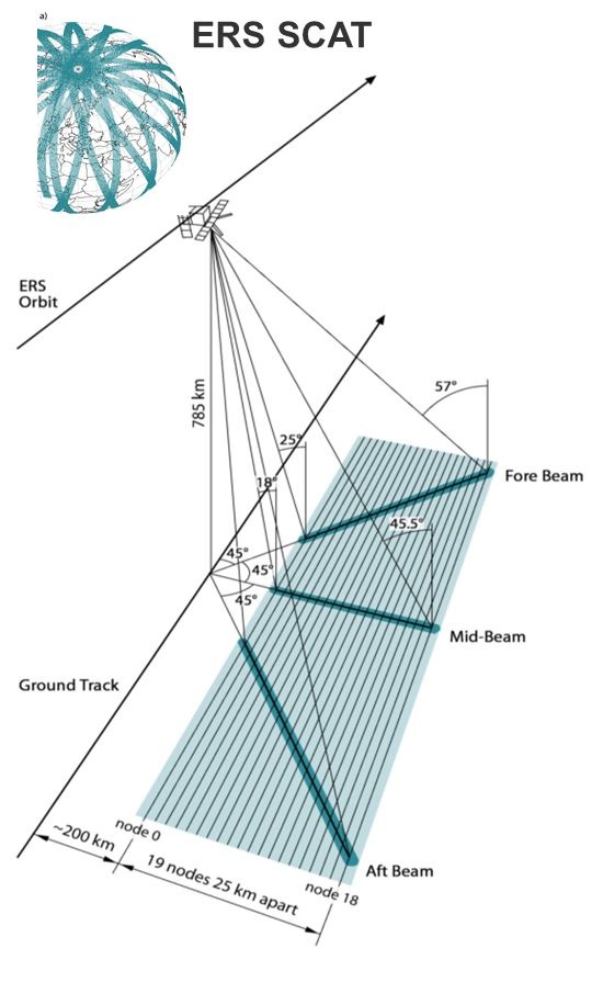
European C-Band Scatterometer
ERS Scatterometers
- $\lambda$=5.7 cm / 5.3 GHz
- VV Polarization
- Resolution: (25) / 50 km
- Daily global coverage: 41%
- Multi-incidence: 18-59°
- 3 Antennas
- Data availability
- ERS-1: 1991-2000
- ERS-2: 1995-2011
METOP ASCAT
- $\lambda$=5.7 cm / 5.3 GHz
- VV Polarization
- Resolution: 25 / 50 km
- Daily global coverage: 82%
- Multi-incidence: 25-65°
- 6 Antennas
- Data availability
- At least 15 years
- METOP-A: since 2006
Instrument Geometry

Observed vs. expected backscatter
The observed backscatter can deviate from the expected theoretical backscatter because of the topography of the Earth's surface.
Topographical mechanisms modulating the backscatter with respect to the azimuth angle are:
- "Sloping Surface Backscattering Targets with Predominant Slope Orientation"
- "Corner Reflectors with Predominant Orientation"
- "Resonant Bragg Scattering"
Scatterometer viewing geometry
Incidence angle $\theta$ vs. local incidence angle $\theta_{L}$:
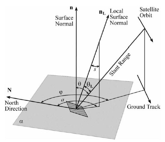
Although the $\sigma^0$ measurement is recorded at the nominal incidence angle $\theta$, the angle determining the backscatter is actually the local incidence angle $\theta_{L}$ because of the local slope of the surface.
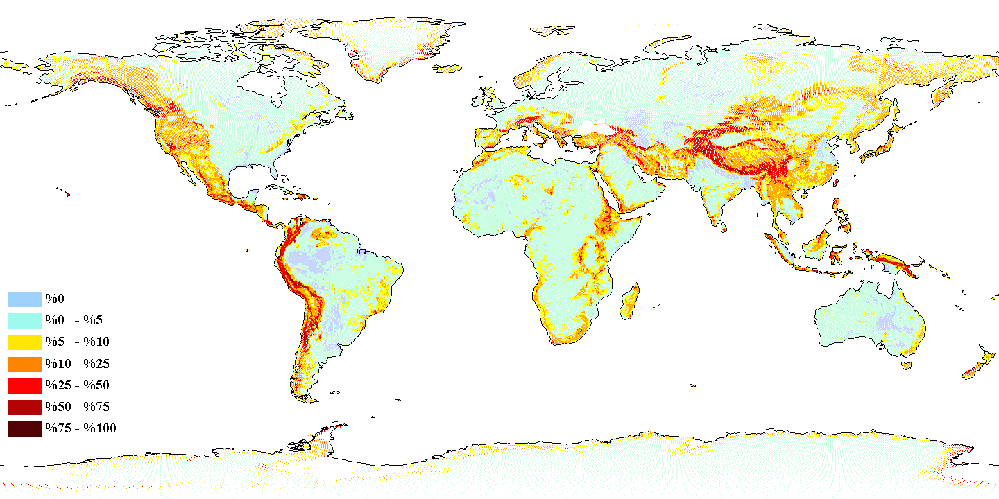
Topographic complexity
- Global elevation data 30 arc-seconds GTOPO30 (USGS)
- Standard deviation of elevation normalized between 0 and 100
Sloping Surface Backscattering Targets with Predominant Slope Orientation
- size of the sloping targets ≥ footprint size (Fig. a)
- e.g. mountain ranges, marginal areas of the Antarctic or Greenlandic ice sheets
- 25/50 km spatial resolution: most places in the world have slope values very close to zero! (however, the standard deviation may be high)
- footprint > size of sloping targets > $\lambda$ (Fig. b, c)
- backscatter is amplified if the satellite is facing the slopes
- e.g. aligned crop fields, sand dunes
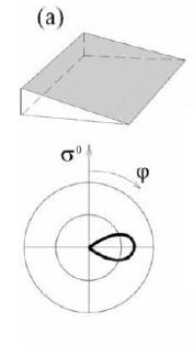

Polar plots of backscatter coeff. $\sigma^0$ versus azimuth angle $\phi$
Corner Reflectors with Predominant Orientation
- aligned scattering targets with very steep local slopes (Fig. d)
possibility of double or multiple "bounce" interaction
backscatter in certain viewing directions from a few point-like targets becomes so high that it can affect the backscatter response over the entire footprint!
e.g. urban areas laid out along a rectangular grid
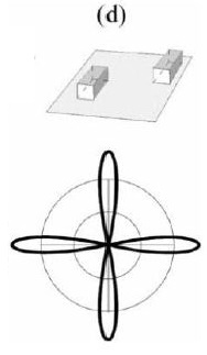
Polar plots of backscatter coeff. $\sigma^0$ versus azimuth angle $\phi$
Resonant Bragg Scattering
size of the sloping targets ≈ footprint size
backscattered waves are subject to constructive interference at certain incidence angles
e.g. reflections from surface ripples on sand dunes
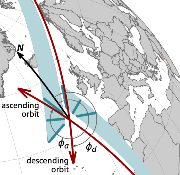
Fore- and aft-beam backscatter I
- $\sigma^0$ is measured at almost the same time and at the same incidence angle, but at two different azimuth angles
- $\sigma^0_{fore}\;-\;\sigma^0_{aft}\;=$ measure of the magnitude of possible azimuthal effects
- Very low values over tropical rainforests
- Extremely high values over sand desert areas (e.g. Sahara, Takalmakan-, Arabian Desert)
Fore- and aft-beam backscatter II
Mean of the differences between fore- and aft-beam taken for ascending overpass (top) and descending overpass (bottom)
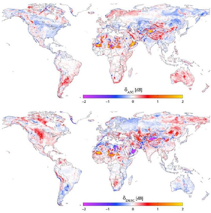
[from Bartalis (2009)]
Azimuthal Anisotropy I
method developed by Bartalis et al. (2006)
statistically expected backscatter value of a target is derived from historically recorded data
azimuthal anisotropy can vary depending on the incidence angle and with the season of the years
number of possible azimuth-incidence combinations:
6 possible azimuth directions
19 possible incidence angles
⇒ 114 possible combinations
Azimuthal Anisotropy II
Enough data must be available
$\delta$ = expected backscatter - measured backscatter
Backscatter measurements can be normalized by adding/subtracting the bias $\delta$
Including seasonal changes: $114\;*\;n$ azimuth-incidence-time combinations ($n$...number of chosen periods)
Azimuthal Anisotropy III
Second order polynomial fitted to the backscatter versus incidence angle relationship, separately for each of the six azimuth angles
Polynomial irrespective of azimuth fitted to all measurements, respresenting the expected backscatter of a target as a function of the incidence angle
⇒ the required azimuthal normalisation biases can be calculated at any incidence angle as the difference between each of the six azimuth polynomials and the seventh, cumulative polynomial