Soil Moisture
Lecture 4: Incidence Angle Normalisation

Funded by:


Backscatter from natural land surfaces
"Scattering": the random distortion of coherent electromagnetic (EM) waves by surface and structures similar to/larger in size than the radar wavelength
any interface separating two media with different dielectric properties affects an incident EM wave
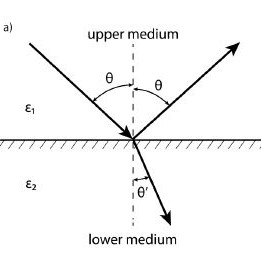
perfectly flat interface ⇒ resulting field: two plane waves (refracted and reflected wave)
Fresnel's law
upper medium: reflected wave, same angle $\theta$ as incident angle
lower medium: refracted wave, angle $\theta'$
Fresnel's law:
$\theta'\;=\;\arcsin{\frac{\sqrt{\varepsilon_2}\sin{\theta}}{\sqrt{\varepsilon_1}}}$
$\varepsilon_{1,\;2}$...dielectric constant of medium 1, 2
Surface Scattering I
occurs if lower medium is uniform and homogenous
scattering only occurs at the surface interface between the upper and the lower medium
dependent on two surface roughness parameters:
- standard deviation of the surface height variations $s$
- surface correlation length $l$
Fraunhofer criterion: a surface is considered smooth if $s\;\lt\;\frac{\lambda}{128\cos(\theta_0)}$
Surface Scattering II
Specular reflection: if the surface interface between two media is smooth compared to the wavelength of the incident wave, the interface acts like a mirror (see Fig. a)
Diffuse reflection: for rougher surface, less energy is reflected in specular direction, and more energy is scattered diffusely (Fig. b-d)

Interesting for us: radiation in sensor direction (= backscatter)
A larger incidence angle automatically means more specular reflection, and the other way round!
Relationship Incidence Angle - Roughness - Backscatter
Surface roughness
Whether a surface appears to be smooth or rough depends on the wavelength of the incident wave.
Rayleigh-criterion: a surface is classified as rough, if the root mean square height $h$ > $\frac{\lambda}{8}*\cos{\theta}$
$\lambda$...wavelength, $\theta$...incidence angle
ACF and correlation length
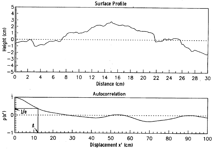
normalised autocorrelation function (ACF) $\rho(x)$
- measure of the similarity between the heights at two points
surface correlation length $l$: the displacement $x'$ for which $\rho(x)$ is equal to $\frac{1}{e}$ (see next slide)
- $l$ is a measure for the statistical independence of two points: if they are separated by a horizontal distance greater than $l$, their heights may be considered to be approximately stastistically independent
perfectly smooth (specular) surface: $l\;=\;\infty$
Surface profile & corresponding ACF
Volume Scattering I
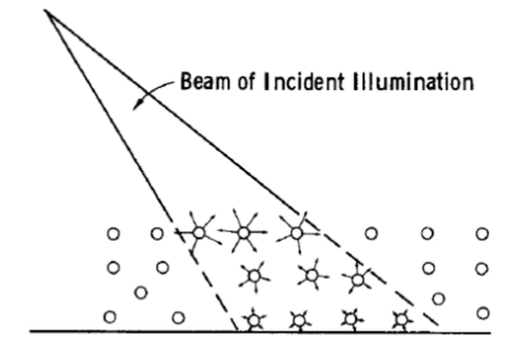
In case of an inhomogeneous medium, scattering can occur within the medium itself.
Dielectric discontinuities within the medium cause absorption and scattering in all directions ⇒ energy loss of the propagating wave
Size, shape and distribution of the individual dielectric discontinuities is more critical than the roughness of the surface boundary
Volume Scattering II
Such inhomogeneities can be leafs, twigs etc. of a vegetation canopy, snow flakes of a dry snow pack, or air bubbles in ice
Relationship Incidence angle - backscatter coefficient I
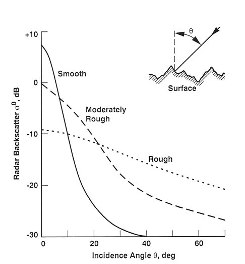
The backscatter coefficient $\sigma^0$ is strongly related to the incidence angle $\theta$:
Increasing incidence angle ⇒ rapidly decreasing backscatter values
Therefore, to compare measurements taken at different incidence angles, an incidence angle normalisation
needs to be applied first!
Relationship Incidence angle - backscatter coefficient II
Main influence factors:
- surface roughness
- amount of biomass
The figure shows the backscatter $\sigma^0$ as a function of the incidence angle for three different biomes.
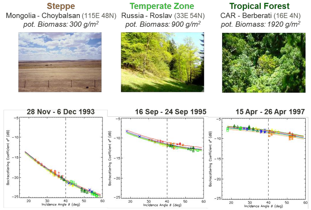
The slope of the curves is indicative for the scattering mechanism taking place at the observed target.
Backscatter incidence angle behaviour
The backscatter incidence angle behaviour can be sufficiently modelled using a second order polynomial:
\begin{equation} \begin{split} \sigma^0(\theta,\;t)\;=\;&\sigma^0(40°,\;t)\;+\;\sigma'(40°,\;t)(\theta\;-\;40°)\;\\ &+\;\frac{1}{2}\sigma''(40°,\;t)(\theta\;-\;40°)^2 \end{split} \end{equation}
- slope $\sigma'(40°,\;t)$ - first derivative of $\sigma^0(\theta)$
- curvature $\sigma''(40°,\;t)$ - second derivative of $\sigma^0(\theta)$
- both parameters are a function of time $t$ and incidence angle $40°$
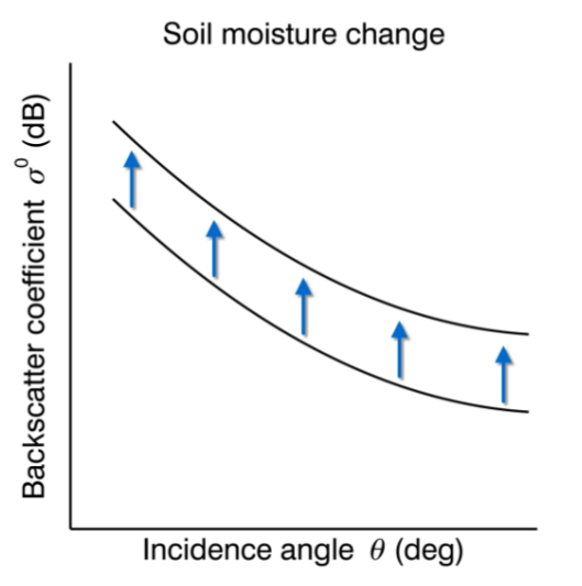
Soil moisture change
Assumption: slope $\sigma'(40°,\;t)$ and curvature $\sigma''(40°,\;t)$ are unaffected by soil moisture variations
⇒ changes in soil moisture are only reflected in the magnitude of the backscatter coefficient $\sigma^0(40°,\;t)$!
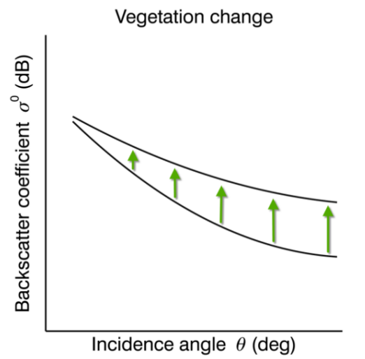
Changes of vegetation or surface roughness
Changes in the slope or curvature show variations in the vegetation phenology or changes in the surface roughness.
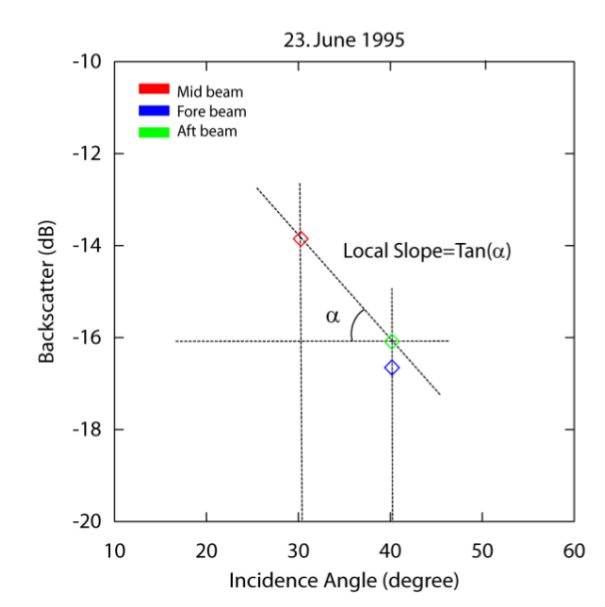
slope and curvature estimation I
ESCAT: 3 beams (fore-, mid-, aft-beam)
estimation of the local slope $\sigma'_L$
each backscatter triplet yields two local slope estimates:
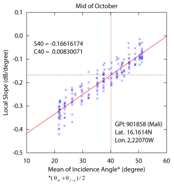
slope and curvature estimation II
regression line fitted to the computed local slopes $\sigma'_L$ aquired during a particular period:
slope and curvature can be obtained from the regression line
slope and curvature estimation III
$\sigma^0$ depends on the incidence angle $\theta$. This dependency is not constant
over the year but changes with soil moisture and vegetation phenology.
⇒ 12 values for slope and curvature are computed for each month of the year
Values for each day: interpolation of the monthly values
Global monthly slope
Compare the slope variability in rainforest areas to that in temperate zones (e.g. Europe or North America)!
Incidence angle normalisation
The incidence angle normalisation can be performed using a full complement of 366 slope $\sigma'(40°,t)$ and curvature
$\sigma''(40°,t)$ values.
Finally, the following equation is used to derive backscatter coefficients normalised to 40° incidence angle
$\sigma^0(40°,t)$:
\begin{equation} \begin{split} \sigma_i^0(40°,t) =\; & \sigma_i^0(\theta,t)\;-\;\sigma'(40°,t)(\theta\;-\;40°) \\ & -\;\frac{1}{2}\sigma''(40°,t)(\theta\;-\;40°)^2 \end{split} \end{equation}